What exactly is Video Feedback?
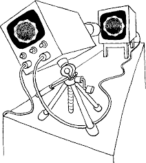
Say that you have a camera and screen that both have the exact same resolution and are both only working in greyscale. In the following diagrams the blue grid will represent what the screen is displaying and the red grid will represent what the camera is seeing, but in a highly quantised manner because I did not have the wherewithal to draw them in 648 by 486. The arrow will represent the mapping from the camera back to the screen and the blue grid on the right will represent what the camera saw on the screen on the left.
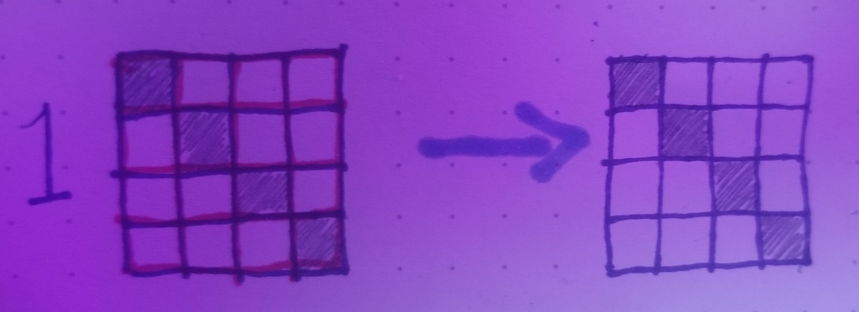
In 1 we have a perfect match between the grids so the diagonal line of black pixels will be perfectly preserved in the mapping. Note that if the camera resolution was higher than the screen resolution by some whole number (for example if the screen was 4x4 and the camera was 8x8) then the line would be perfectly preserved but not if the resolution was some fractional resolution higher (for example the screen was 4x4 and the camera was 6x6). Try working through this last example on your own and you will find out why and also gain some intuition on the concept of aliasing!
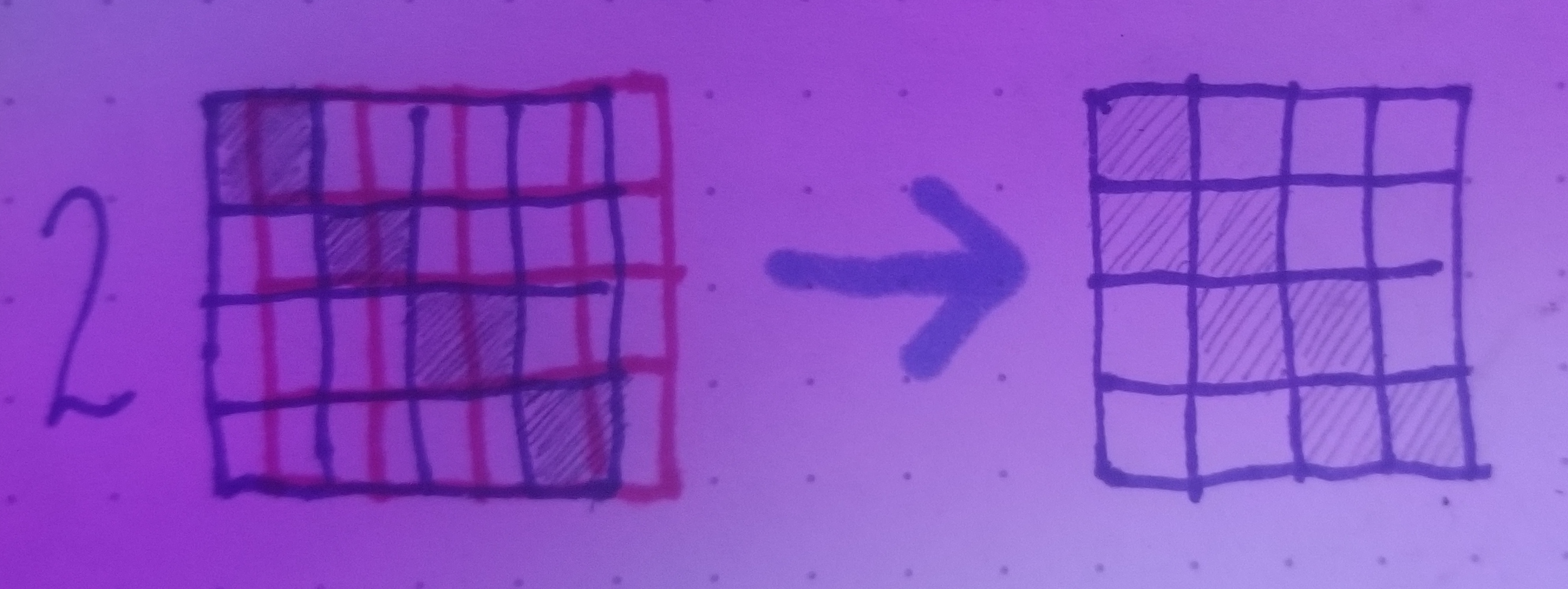
In 2 we have the camera grid shifted over to the right by one half gridstep. Since the grids represent the smallest discrete values that the screen and the camera can display and detect respectively we have to stop and figure out what it means when a camera has to map a cell that is 50 percent black and 50 percent white to a single cell. Luckily this is a pretty simple operation to represent mathematically, the camera basically just averages out the values between the two cells so this will get mapped to the value of grey that is exactly between black and white. Note that this smears the black line into a greyscale line over to the left. So a right shift of the camera will result in leftwards motion on the screen! Lets next try to imagine what will happen in the next couple of frames if we keep the camera in the same position. Next iteration the original diagonal line will be 1/4 of the darkness as it was originally, the newer diagonal line to the left of it will be the same 1/2 grey as before, and there will be one more new diagonal line of 1/4 greyscale to the left of this newer one. We can extrapolate from this that the original line will fade out soon and that the half greyscale line will creep its way over to the left until it disappears and the screen is entirely white.

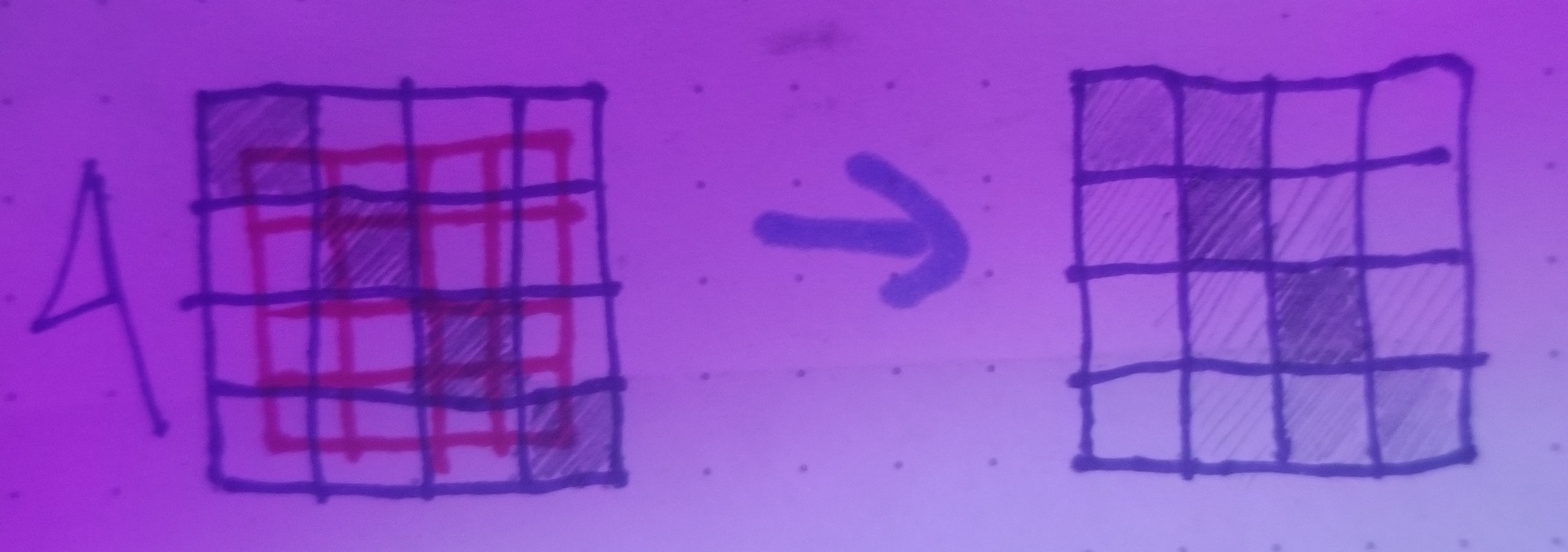
In 3 the camera grid is shifted both to the left and up. In the map we have the original diagonal line mapped to one of 1/4 greyscale, another diagonal line to the lower left at 1/2 greyscale and one more to the lower left of that at 1/4 greyscale. We can extrapolate from this that with further iterations the movement will be both to the left and downwards and have a slightly different pace and amount of greyscale than in example 2
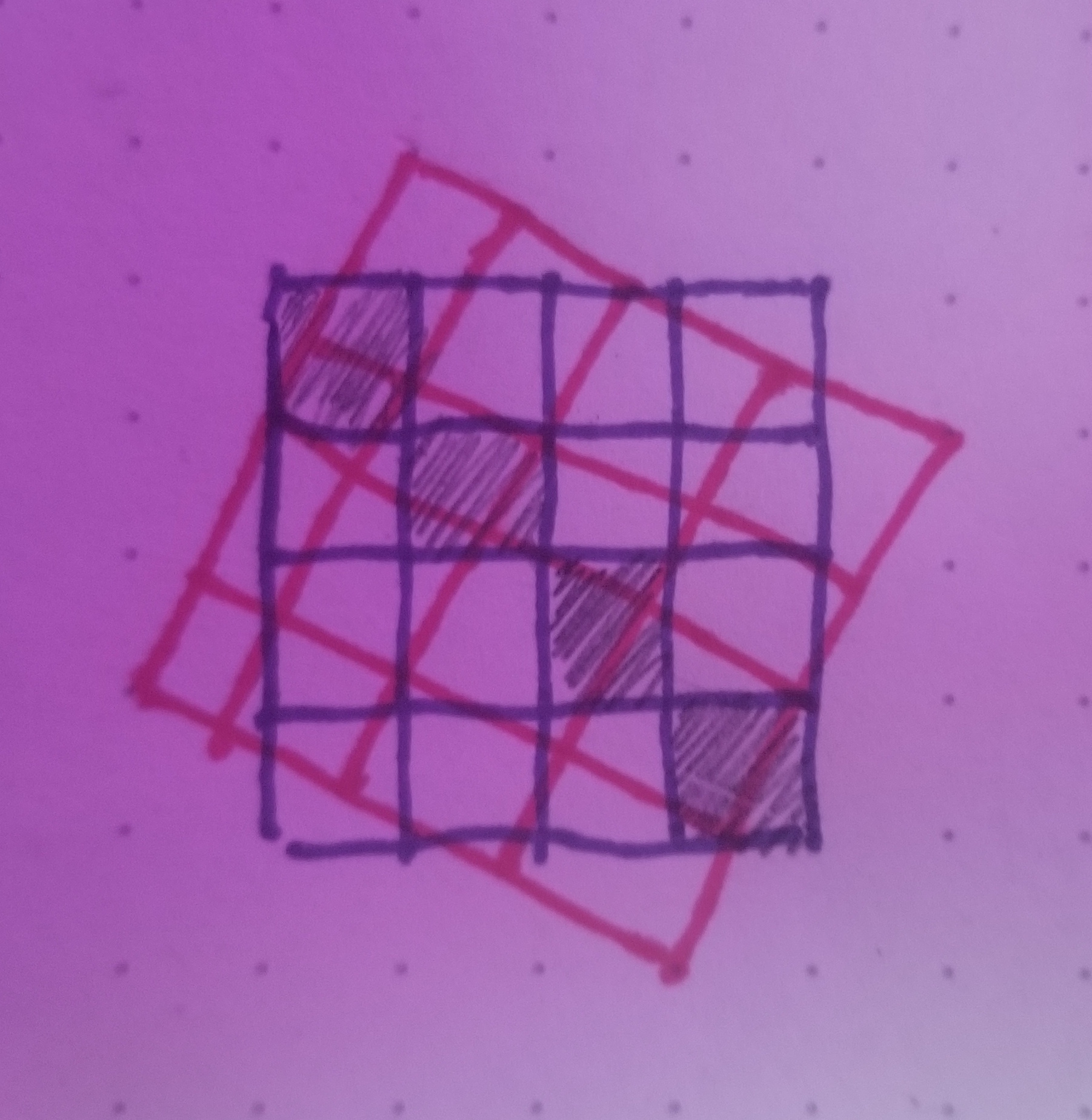
In 4 we have the camera zoomed into the screen. This will result in a smearing around the corners of the diagonal and a fainter smearing near the middle. If we had a larger resolution grid we could more easily see that what is happening is blowing up the pixels in the center of the screen to a smeared out aliased image of itself. Note that the middle two pixels stay the exact same concentration of black in this map! Further iterations will preserve these two pixels at full black while smearing around greyscale stuff around everywhere else, creating a sensation that our brains and eyes will combine to see as movement shooting out from the center of the screen.

in 5 we have the camera zoomed out from the screen. If we had a higher resolution grid we would more obviously see that our original image is being replicated as a lower resolution version of itself in the center of the screen. Further iterations will create the sensation of of an image receding into a vanishing point at the center of the screen. Note that while in this mathematically ideal version we assume there is nothing to see on the outside of the screen but in an actual screen the camera will be picking up bits of the border of the screen and feeding that information into each map as well.

These final two examples are for you to work out on your own! They represent a shear and a rotation respectively.
So what was the common operation we performed in each of these maps? Each time we calculate a weighted average of all of the overlapping pixels that the camera saw with weights being assigned as a function of how much of each pixel overlapped with the cameras grid. In image processing when we calculate a new value of a pixel by performing a weighted average of its neighboring pixels we call this a convolution. Blurs and sharpens are achieved through use of convolutions.
(You can skip this part if you don't like to read math )
In differential calculus we call this kind of map a laplacian operator. The laplacian operator is a measure of divergence of a gradient. In functions of 2 variables a gradient is a generalization of taking a derivative. In functions of one variable a derivative of a function returns another function which measures the slope of the original function at every point. So in two dimensions a derivative is represented by what we call a flow field of vectors. When we measure the divergence of this flow field we are returned with not a field of vectors but a field of numbers, each of which measures how much the rate of change is changing. So performing an operation which iterates a laplacian operator on its output will result in a pattern of behavior in which larger rates of change will be amplified each step by how much they change each step! Fun fact, you if you read through to this point you just have managed to understand a small bit of differential calculus without having to do any calculus at all! Thats yet another interesting application of video feedback: how simply you can model and represent complex mathematical structures without having to program anything with differential equations!.
This map translates very well to cellular automata systems. In cellular automata instead of directly computing weighted averages of our neighborhood we instead have a rule set that maps each permutation of states of the neighborhood to a new value for the pixel. Much of my original research and experimenting with digital feedback systems began using the cellular automata model. I would reccomend at least browsing through the first handful of chapters of Steven Wolframs A New Kind of Science if you are interested in working with these models, there is a wealth of useful information and some beautiful CA artwork throughout that book.
The camera feedback kind of convolution differs from the cellular automata and laplacian operator concepts in a significant way. We can move the camera around while its pointed at the screen. In terms of convolutions what this means is that we can change the neighborhoods and weights of the averages for each convolution on the fly! This differs very strongly from the cellular automata world where one just writes down some fixed rule sets and seeds a grid and then passively lets the behavior do what it has to do. In camera feedback we have the ability to steer these strange attractor systems around in phase space! So if we want to properly model this kind of behavior in a system we need to make sure that we can change our neighborhoods and weights at any point but ideally in a continuous manner.
While understanding the convolution aspect of the feedback is crucial, this is only part of the actual map that happens when we are doing camera feedback! It was very useful to do a mathematically ideal reduction of the behavior to get a feel for convolutions, in the physical reality of camera screen feedback there is a lot more happening in many stages of the signal flow. First off there is the kind of screen involved! If it is a crt we have to also think about how the phosphors themselves have an fuzzy blurriness to them on an individual basis which results in a bit of inherent blur. There is the specularity of the screen itself, maybe there is another light on in the room somewhere and it is reflecting a bit of that that the camera picks up every time. Maybe there is something slightly awry with a part of the aperture grill in the CRT so some of the electrons are not deflected properly and results in dead pixels or multiple phosphors firing on the same part of the screen. Perhaps you are using a camera that only has HDMI out and you have to downscale the signal to 800 by 600 using an inexpensive downscaler in the chain. Perhaps there is a large dog that lives upstairs and every time it runs across the living room it shakes your camera.
It would be pathological to attempt to list and attempt to mathematically represent ever single possible environmental aspect that can affect this signal flow. However we are not interested in direct emulation of an environment at this point, we are more concerned with figuring out how to replicate the general class of behavior. In my experiments I've found that it is sufficient to just add some sort of nonlinear map to the convolution at each step!
What exactly is a linear map?
There is a simple way to think about linear and nonlinear maps using graphs! A linear map graphs to a straight line and a nonlinear map is just literally every map that doesn't.

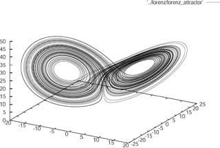
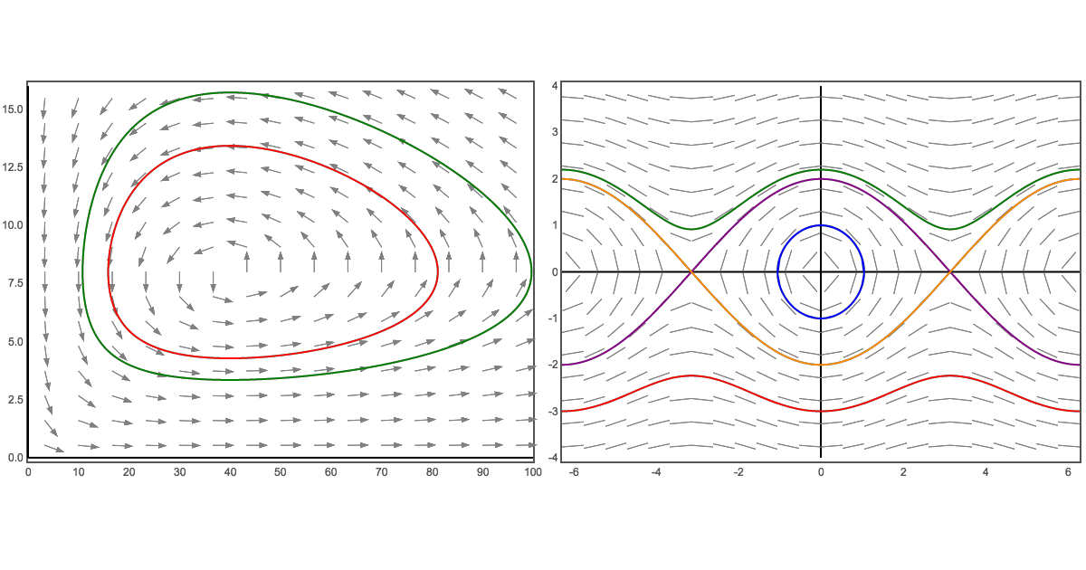
At this point you may be thinking “ok enough with the mathematical digressions just tell me what kind of nonlinear maps to use and how to use them.” To answer the first I will now go on another mathematical digression. One of the developers of chaos theory, Michael Figenbaum discovered very compelling pattern that linked nonlinear iterative maps. The canonical nonlinear iterative map in chaos theory history was the logistic function x_n+1=r*x_n*(1-x_n) for some constant r, which was used to model populations. When people examined the varying dynamics of this map as they varied the parameter r they found that as r grew larger and larger the patterns of fluctuation in the populations began to trace out a very beguiling design.
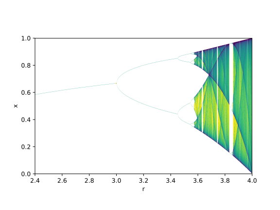
Above we have a bifurcation map of the function x_n+1=r*sin(x_n).
And here is a bifurcation map of the function x_n+1=sin(x_n+π)+r.
Notice the pattern of shaded banding in each of these pictures. Without going in to much more mathematics I will only say that these patterns represent structures in nonlinear dynamic systems and that any nonlinear iterative system will contain a similar set of structures. This was a very long winded way to say that in the grand scheme of things it doesn’t really matter what specific nonlinear map you use, they will all give you interesting patterns when used in feedback systems! If you are writing something in code or using a visual coding environment there should be access to the basic transcendental functions (sin, cos, exp, log) and I would recommend playing around with all of them to get a flavor for how they work!
Unfortunately I don’t even have a mathematical digression to help with the second question. The actual implementation of nonlinearities with convolutions in feedback systems is something that really just needs to be experimented with because thats how chaotic systems work! They are by nature difficult to predict.
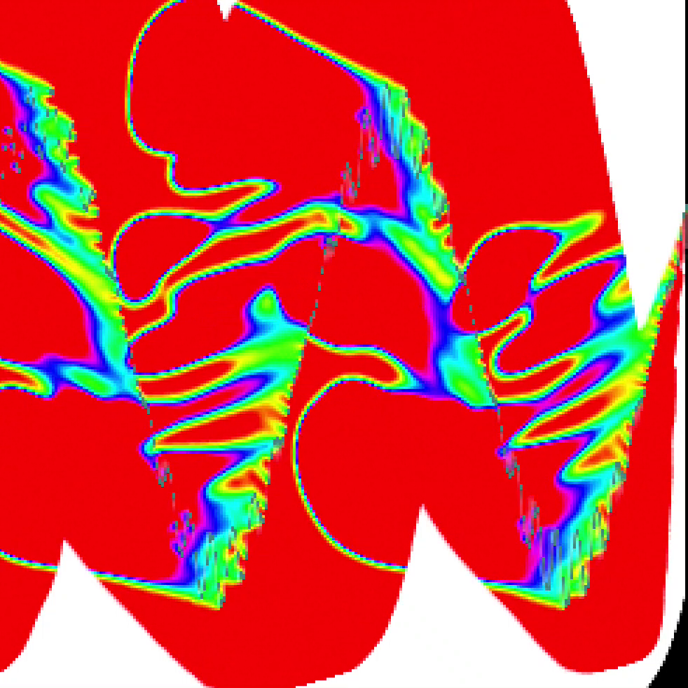
At the above link you can find an example of some coarse grained video feedback synthesis in action that I designed in Processing. If you take a look at the code you can see that there are three independent feedback channels for hue, saturation, and brightness in this system and each is working with a slightly different kind of convolution and some only have conditional nonlinearities. I don’t really have any concrete explanation for why I ended up with these values other than I did a lot of testing and they seemed to have great results!
hHere is another feedback system I designed in openFrameworks. If you take a look at the iterative maps involved you will see some crazy things happening. I pretty much forgot most of the details but there was the ability to switch back and forth between a discrete heat diffusion model and a discrete reaction diffusion model which was pretty fun!

https://github.com/ex-zee-ex/VIDEO_WAAAVES_2
In the most recent feedback synthesis program that I am continuing to develop you can find some very concrete examples of effects of nonlinear maps. There are controls for the hue channel in the framebuffer feedback processing part of the gui that are labeled hue offset and huelfo. These two parameters are an implementation of the map x_n=sin(x_n) + c! If you examine the feedback color processing part of the code you will also notice that there are currently no nonlinearities in the saturation and brightness channels. This is primarily because I have not discovered the proper way to implement them in this system as of yet! There seems to be a psychovisual aspect to the different ways that human brains process the qualities of brightness and saturation that is qualitatively different from how human brains process hue which for me means that I just need to do more applied research in this zone to find the best system of controls in these realms!

https://github.com/ex-zee-ex/intro_to_digital_feedback
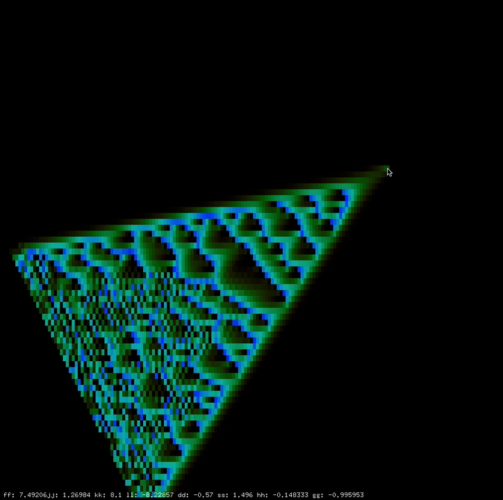
If you made it this far then you have consumed what I would think is a healthy amount of information to have in order to begin experimenting with digital feedback systems! The above link is to a very basic outline of a digital feedback system in openFrameworks and glsl, the signal path of a ping pong framebuffer in openFrameworks and a simple convolution in the shader.frag is all set up so there is a wide open range to explore! The above picture was taken from video generated by modifying only 2 lines of code.
If you enjoy the mathematical perspective on video feedback systems I recomend this paper which takes a more in depth look at the specific physical systems of cameras and displays used at the time and how the camera feedback system contrasts with a reaction diffusion system. The delightful video companion to this paper is below.

If you appreciate the public domain open source software and educational materials I provide and can afford to spare some cash it is highly appreciated! The more donations I recieve the more time I have to spend on developing these resources! Please also consider subscribing to my patreon page as small amounts of regular income are appreciated as well!